An Experiment on DFT --- validation and application of DFT in Python
[Abstract] This work presents a basic experiment exploring Discrete Fourier Transform (DFT) using Python's NumPy library. It begins by establishing the foundation of the DFT equation and then leverage the NumPy fft package to perform real-world spectrum analysis. While this experiment focuses on fundamental techniques, attempts at pitch detection and filtering offer a glimpse into the vast potential of signal processing.
INTRODUCTION
Fourier Transform (FT) is a cornerstone of signal processing, holding immense significance in various engineering applications. Derived from Fourier series and continuous signal analysis, Discrete Fourier Transform (DFT) specifically caters to discrete signals. In digital music, all sounds, regardless of their apparent smoothness, are ultimately represented by sequences of discrete samples. This process, akin to capturing sound with a microphone and converting it to digital data, is called Analog-to-Digital Conversion (ADC).
The visual representation of sound is often depicted as a waveform in the time domain. This representation is intuitive for listeners because the horizontal axis represents time and the vertical axis represents corresponding amplitude. Even without prior knowledge, one can readily grasp the shape of the waveform. However, a crucial aspect of sound – frequency – remains absent. Frequency plays a vital role in how the human ear perceives "tone color."
Fourier Transform empowers us to analyze complex sounds by deconstructing them into simpler components. It leverages the concept of decomposing general functions into trigonometric or exponential functions with distinct frequencies.[1] In the context of digital audio, this translates to representing any complex wave as the sum of fundamental sine waves, each characterized by a specific amplitude and phase. Applying this theorem to sound processing leads to the development of the powerful and widely used Discrete Fourier Transform (DFT). The brilliance of DFT lies in its ability to transform a time-domain signal into its frequency domain representation (spectrum) using a relatively straightforward equation.
PART I. Validate DFT
Step 1 - DFT Equation
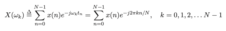
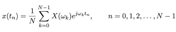
For a signal x, DFT may be defined by
where
$ t_n= nT $, $ω_k= 2πk/N$
$ T = 1/fs$ (normalized as 1, usually omitted); fs is sampling rate.
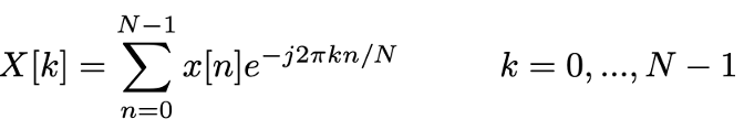
or in a simpler way
where $x[n]$ is the input signal.
Specifically, $n$ is time index of signal $x$ which is a discrete sequence (indicates the nth sampling instance). For a certain $n$, $x[n]$ refers to its corresponding value.
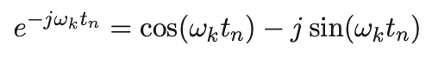
As an important part of the equation, the expansion of the complex exponential (Euler’s formula) is always following the main equation above.
Instead of round bracket ( ), the square bracket [ ] is prefered considering the later usage in Python since it's implying the signal as a sequence/array. It’s typical to use square bracket for indexing in Python.
The capital N is the number of samples or the length of signal, and the lowercase n is time index denoting current sample. A signal with length of N means it contains N discrete samples. Therefore, time index n ∈ [0,N). The index starts from 0, that's why we put "N-1" on top of the big sigma.
$X[k]$ on the left side is certaintly the result obtained from DFT. This is the spectrum of signal x encoded both the information of amplitude and phase. The k is used as frequency index denoting current frequency sample. For a certain k, $X[k]$ indicates a spectrum at a radian frequency . DFT only transforms a signal into its spectrum and won't change any of it, so the resulting data will have the same length as the input signal. Therefore, frequency index $k ∈ [0,N)$ just as $n$.
The complex exponential part is also called the “kernel” of DFT which is the basis function. It's actually a complex sinusoid which could be expressed as a cosine (real) and sine (imaginary) as above.
$ω_k$ is defined as the kth frequency sample in radian per second ($ω_k=2πk/N$) . According to the basic idea of DFT that transform time domain sampling into frequency domain sampling, $k$ denotes each one of the possible frequencies. $ω$ is conventionally used as radian frequency ($ω=2πf$) in sinusoidal functions or circular motion denotation.
So the two main parts of the equation -- input signal and complex sinusoid are multiplied together sample by sample, and eventually summed together. With the understanding of DFT equation, it’s possible to use Python to program each part of the formula. But I can't put it into a general function yet, since it's impossible to compute a summation of an unknown sequence. How does this measuring really happen? This brought me to a deeper view of DFT.
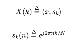
Step 2 - DFT and Vector Dot Product
The "multiplication and summation" operation in DFT feels familiar. It closely resembles the concept of vector dot product, also known as scalar product or inner product. In linear algebra, the dot product involves multiplying corresponding elements of two vectors and then summing them to obtain a single scalar value. Geometrically, it represents the magnitude of one vector multiplied by the projection of another vector onto it (|a| |b| cosθ). This connection was instrumental when I first grasped the idea of signals as vectors.
Fourier's theorem tells us that a complex wave can be decomposed into a sum of simpler sine waves. From a geometric perspective, in an N-dimensional space, each sine wave component contributes a single value (zero or non-zero) to the final sound vector. This allows us to represent any sound using coordinates like [value1, value2, ..., valueN]. Essentially, the sound becomes a vector – an arrow in a high-dimensional space. In this vector space, each dimension's unit is a basis sine wave with a specific frequency. In the real world, sampling rates of 44.1 kHz or higher theoretically capture all frequencies audible to the human ear (limited by the Nyquist frequency of 22.05 kHz).
Therefore, applying DFT to a sound can be interpreted as a "mapping" process. Considering the projection aspect of the inner product, DFT maps each spectral component in the sound (input signal) onto all possible frequencies within the range covered by the sampling rate. The "sample by sample" multiplication is the core of this mapping. If a particular frequency is absent in the sound (meaning there's no energy at that frequency), the projection will be zero, resulting in its exclusion from the final spectrum.
The algebraic definition of the complex-valued inner product aligns with this concept. It involves summing the product of each component in one vector with the complex conjugate of the corresponding component in the other vector.
This provides an alternative way to understand DFT.
Now I can implement these theories in Python.
Step 3 - experiment DFT in Python
a. Exploring the Complex Exponential
The key to understand DFT is the kernel of the equation. Say $S_k$ denotes the complex
exponentials, its conjugate is denoted as $\overline{S_k}$ . For a signal with length of N=8, for instance, I'll need 8 basis sines. Thus for $n=0,1,2...7$, and $k=0,1,2...7$. According to the formula of $\overline{S_k}$ , when $k=0$, $\overline{S_0}=cos(2π0n/4) - jsin(2π0n/4)$, multiply each $n$ to it,
%matplotlib notebook
import numpy as np
import matplotlib.pyplot as plt

N = 8
k = 0

s0 = np.zeros(8,dtype=np.complex64) #create a container for s0 data

for n in range(8):
    s = np.cos(2*np.pi*k*n/N) - 1j*np.sin(2*np.pi*k*n/N)
    s = np.around(s,1)
    s0[n] = s
print(s0)
I got the coordinates of the basis sine $\overline{S_0}: [1. 1. 1. 1. 1. 1. 1. 1.]$
For $k=1$, multiply each $n$ to it:
k=1
s1 = np.zeros(8,dtype=np.complex64)
for n in range(8):
    s = np.cos(2*np.pi*k*n/N) - 1j*np.sin(2*np.pi*k*n/N)
    s = np.around(s,1)
    s1[n] = s

print(s1)
N = 8
for k in range(8):
    sk = np.zeros(8,dtype=np.complex64)
    for n in range(8):
        s = np.cos(2*np.pi*k*n/N) - 1j*np.sin(2*np.pi*k*n/N)
        s = np.around(s,1)
        sk[n] = s
    print('s%d ='% k,sk)
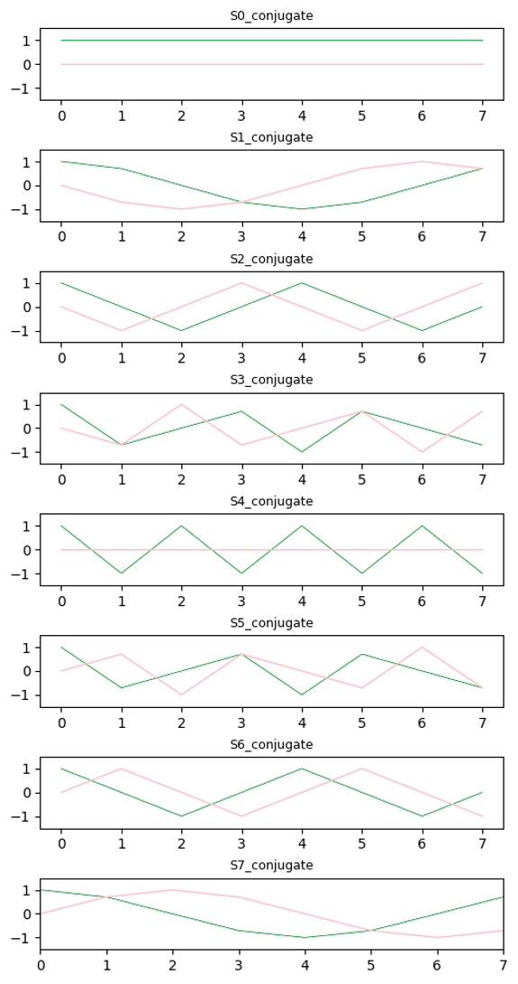
To plot each complex sinusoid as a pair of cosine and sine:
N = 8
n = np.arange(8)
figure,axis = plt.subplots(8,1,figsize=[6,12], sharey=True) #8rows 1 colunm
plt.axis([0,7,-1.5,1.5]) #set y-axis broader than the peak
plt.subplots_adjust(hspace = 0.7) #height space
row = 0
for k in range(8):
    cos = np.cos(2*np.pi*k*n/N)
    sin = - 1j*np.sin(2*np.pi*k*n/N)
    sin = np.imag(sin) #keep the coefficent of j only

    axis[row].plot(cos,color='green',lw=0.5)
    axis[row].plot(sin,color='pink',lw=1)
    axis[row].set_title('S%d_conjugate'% k, fontsize=9)
    row += 1
Surprisingly, the results from plotting eight complex sines revealed a symmetrical pattern. The first component represents the DC component in physics, which is a constant value. As the frequency index increases, the periods in the resulting graph become progressively shorter (higher frequencies). However, this increase reaches a turning point in the middle and starts reversing. Eventually, the frequency reaches 1 again.
This symmetry is a fundamental property of the Discrete Fourier Transform. The "backward" portion of the spectrum is referred to as negative frequencies. These negative frequencies can be interpreted as representing circular motion in the opposite direction. Imagine a phasor rotating counter-clockwise for positive frequencies. Negative frequencies then correspond to a phasor rotating clockwise. This concept plays a crucial role in understanding Nyquist theory.
[notes] Based on the analysis of trigonometric functions and Euler's formula, it becomes clear that any sinusoidal signal can be decomposed into a cosine and a sine component. From a geometric perspective, these components can be visualized as projections of circular motion (in a 3D space) onto the complex plane. The real part in Euler's formula represents the projection of this circular motion onto the real axis (vs. time), resulting in a cosine function. Similarly, the imaginary part represents the projection onto the imaginary axis (vs. time), resulting in a sine function.
b. Implementing the Inner Product
Now that I have eight basis vectors representing sine waves, I can use them to calculate the inner product with a signal for a DFT operation of length N=8. Recall that the inner product of vectors A and B can be expressed as A' ⋅ B = |A| * Proj_A(B), where A' is the conjugate of A and Proj_A(B) represents the projection of B onto A. In the context of DFT, we are essentially mapping the signal (B) onto the basis vectors (A).
Python's NumPy library provides a numpy.dot() function for calculating the dot product, which is equivalent to the inner product for real-valued vectors. Since I've already calculated the complex conjugates of the basis vectors, I can directly use numpy.dot() to compute the inner product between the signal and each basis vector.
However, before proceeding, I need a test signal. With only eight basis vectors at our disposal, choosing a suitable signal becomes crucial. Fortunately, sine functions are simple and well-understood. We can create a test signal using the sinusoidal function: $x(t)=Asin(ωt+φ)$
def sinusoid(f0,dur,fs,A=1,phi=0):
"""generate a simple sinewave
--------params--------
f0=initial frequency; dur=duration of signal; fs=sampling frequency.
A=amplitude; phi=phase shift
--------return---------
sinusoid (array)
"""
N = fs*dur # length of the signal / number of samples
t = np.arange(0,dur,1/fs) # discrete time seq
xs = A * np.sin(2*np.pi*f0*t+phi)
plt.figure(figsize=(4,2))
plt.plot(t,xs)
plt.xlabel('time')
plt.ylabel('amp')
plt.title('little signal to be analyzed',fontsize=8)
return xs
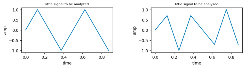
x02 = sinusoid(2,1,8)
x03 = sinusoid(3,1,8)
While the low sampling rate results in a less visually appealing representation of the sine wave, the key aspect lies in the accurate portrayal of the periods in the plots. This is crucial for the inner product calculation.
Now it's time for inner product coming to the stage.
#operating inner product of sk with signal x02
N = 8
t = np.arange(8)
plt.figure()
for k in range(8):
    sk = np.zeros(8,dtype=np.complex64)
    for n in range(8):
        s = np.cos(2*np.pi*k*n/N) - 1j*np.sin(2*np.pi*k*n/N)
        s = np.around(s,1)
        sk[n] = s   #calculate each sk and store it
    product = np.abs(np.dot(sk,x02))   #magnitude of the value of inner product
    print(np.around(product,1),end='  ')

    plt.stem(k,product)
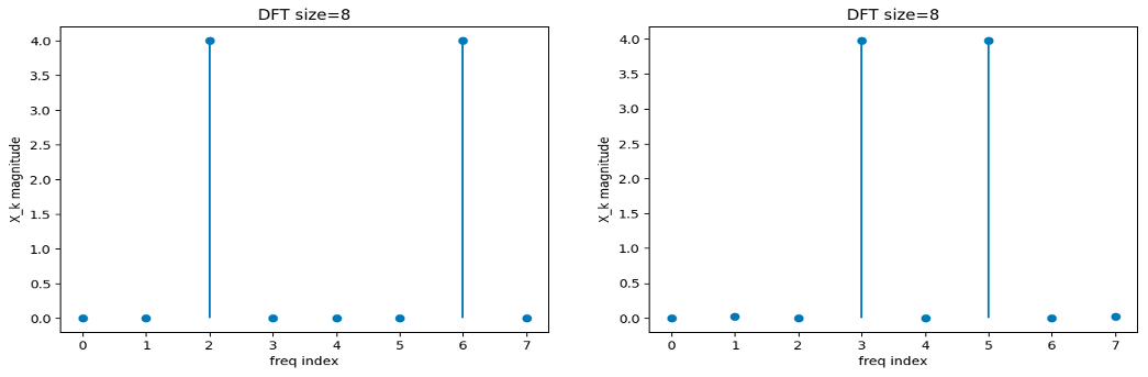
The inner product calculations for signals x02 and x03 resulted in the following outputs, respectively:
x02: [0.0, 0.0, 4.0, 0.0, 0.0, 0.0, 4.0, 0.0]
x03: [0.0, 0.0, 0.0, 4.0, 0.0, 4.0, 0.0, 0.0]
These results demonstrate the expected symmetry in the DFT spectrum, confirming the theoretical concept. However, for the signal x03 with a frequency of 3 and a sampling rate of 8, the limitations become apparent. The low sampling rate leads to a poorly represented sine wave in the time domain and the spectrum analysis is also affected. Increasing the signal's frequency further would likely result in aliasing. This practical example reinforces our understanding of aliasing in digital sampling.
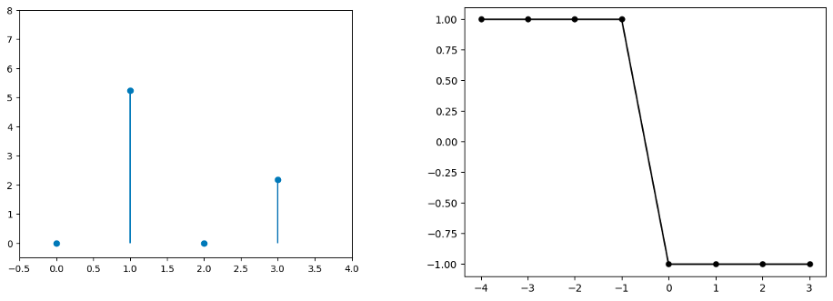
Moving on to a Square Wave
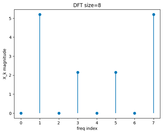
Having explored the behavior with simple sine waves, let's now investigate a richer signal. This new signal x has the following values: [1, 1, 1, 1, -1, -1, -1, -1]. Based on the data points, this appears to be a square wave. Applying the same DFT process, I got the spectrum:
Therefore, the signal contains two frequencies at k=1 and k=3. Just as what we've already known, the square wave contains fundamental frequency and its odd harmonics.
c. Verifying DFT with Inverse DFT (IDFT)
Since DFT transforms a signal from the time domain to the frequency domain and theoretically preserves the information, it should be possible to recover the original signal using an inverse operation. Fortunately, the Inverse Discrete Fourier Transform (IDFT) equation is relatively straightforward.
Let's use the square wave signal as a test case to perform a complete DFT and IDFT process. The code for this will require some modifications to account for the inverse operation. To ensure accuracy, I'll avoid rounding and absolute value conversions during the calculations. Additionally, I use a more convenient indexing scheme of [-N/2, N/2] that reflects the symmetry of the spectrum around zero. The resulting plots will showcase the transformed frequency domain and the reconstructed time-domain signal.
x = np.ones(8)
x[4:] = -1

N = 8
Xk = np.array([])
k_idx = np.arange(-N/2,N/2)
sig_idx = k_idx[:]                 #keep them independent to avoid any further ambiguousness
plt.figure()
for k in k_idx:                    #[-4,-3,-2,-1,0,1,2,3]
    sk = np.array([])
    for n in np.arange(-N/2,N/2):
        s = np.cos(2*np.pi*k*n/N)-1j*np.sin(2*np.pi*k*n/N)
        sk = np.append(sk,s)
    Xk_data = np.dot(sk,x)
    Xk = np.append(Xk,Xk_data)      #spectrum X[k]

    plt.stem(k, np.abs(Xk_data))
    plt.axis([-0.5,N/2,-0.5,N])     #for a natural viewing, the axis need more space
plt.show()

#inverse DFT
xn = np.array([])
for n in np.arange(-N/2,N/2):
    sk_cj = np.array([])
    for k in np.arange(-N/2,N/2):
        s_cj = np.cos(2*np.pi*k*n/N)+1j*np.sin(2*np.pi*k*n/N)    #conjugate of the kernel of DFT
        sk_cj = np.append(sk_cj, s_cj)
    xn_data = np.dot(Xk,sk_cj)/N
    xn = np.append(xn,xn_data)

plt.figure()
plt.plot(sig_idx,np.real(xn),marker='.',markersize=10,color='k')
plt.show()
[Notes on Data Types and Accuracy] It's important to consider data types for numerical accuracy. While NumPy's default complex data type (complex128) offers higher precision, I initially used complex64 to avoid cumbersome complex number representations (a misconception). This approach, however, led to inaccurate results during IDFT due to insufficient resolution for the calculations. As a reminder, rounding errors can accumulate during computations, and choosing the appropriate data type is crucial. Later, when I repeated the IDFT operation with the default complex128 data type, the recovered signal matched the original square wave perfectly.
d. Applying DFT on More Signals
This exploration with the limited set of basis vectors has provided a solid foundation for understanding DFT. Now, let's create a more general-purpose function to handle various sound signals.
As a quick test, I implemented a basic DFT function using a nested loop for clarity.
N = len(x)
Xk = np.array([])
plt.figure()
for k in range(8):
    sk = np.zeros(8,dtype=np.complex_)
    for n in range(8):
        e = np.exp(-1j*2*np.pi*n*k/N)
        sk[n] = e
    Xk_data = np.dot(sk,x)
    Xk = np.append(Xk,Xk_data)
    Xkmag = np.abs(Xk)
    plt.stem(Xkmag)
The function successfully processed three test signals. However, the current implementation suffers from readability issues due to the nested loop structure. Ideally, I want the code to more explicitly reflect the mathematical operations involved in DFT.
The core idea behind DFT is essentially calculating the inner product of the signal vector with each basis vector (complex exponential) in the frequency domain. In mathematical terms, this translates to multiplying the signal sequence with each exponential term. Traditionally, DFT is often implemented using nested loops. However, NumPy offers powerful vectorized operations that can achieve the same result more efficiently and concisely.
A= np.array([0,1,2,3])
B = np.array([0,1,2,3]).reshape(4,1)
print(A*B)
[[0 0 0 0]
 [0 1 2 3]
 [0 2 4 6]
 [0 3 6 9]]
By leveraging these vectorized operations, we can eliminate the nested loop structure and improve the code's readability.
Function Design
The following code snippet demonstrates a more streamlined DFT function that utilizes vectorized operations:
def simpleDFT(x):
    N = len(x)                    #length of signal
    n = np.arange(N)              #time indices
    k = n.reshape(N,1)            #freq index
    #print(n*k)
    e = np.exp(-1j*2*np.pi*n*k/N) #basis sinusoid coordinates
    Xkmag = np.abs(np.dot(e,x))   #DFT result and convert the absolute value
    return Xkmag
simpleDFT(x03)
To plot a spectrum and also give it an optional zoom-in view to check the detail:
def spectr(Xkmag,fs,zoom_start=0,zoom_end=None):
    N = len(Xkmag)
    n = np.arange(N)
    plt.figure(figsize=[10,4])
    if zoom_end==None:
        plt.stem(Xkmag[zoom_start:],linefmt='green',basefmt=' ',markerfmt='.')
    else:
        plt.stem(Xkmag [zoom_start:zoom_end],linefmt='green',basefmt=' ',markerfmt='.')

    plt.title('DFT result')
    plt.xlabel('freq Hertz')
    plt.ylabel('amp')
    plt.show()
While I've successfully obtained the DFT results, the horizontal axis (k) doesn't directly correspond to actual frequencies. It represents a discrete set of indices ranging from 0 to N-1, where N is the length of the input signal.
However, we can translate these indices into meaningful frequencies. A value at a particular index (k) indicates the presence of a frequency component in the signal. For example, the value at k=57 suggests a frequency component with some energy.
Here's how to interpret the k value:
Frequency Resolution: The total number of k values (N) represents the frequency resolution of the DFT. It's related to the sampling rate and the signal duration: $N = \text{sampling rate} * \text{duration}$.
Normalized Frequency: The index k is essentially a position within the spectrum (length N). To convert this position into a normalized frequency, we calculate $k/N$. This value represents a fraction of the total bandwidth (determined by the sampling rate).
Actual Frequency: Finally, to obtain the actual frequency, we multiply the normalized frequency by the sampling rate: $\text{frequency} = (k / N) * \text{sampling rate}$.
Interestingly, from a mathematical perspective, the sampling rate cancels out when calculating the actual frequency using $k/\text{duration}$ (k being the index and duration being the signal length). In this specific case, with k=57 and duration=3, the frequency becomes 57 / 3 = 19 Hz. This applies to all other frequency components identified in the spectrum.
Then, a modified version of spectr() function:
def spectr(Xkmag,fs,freq_start=0,freq_end=None):
    """take DFT result(magnitude) as given data and plot out the spectrum.
    fs = sampling rate of original signal
    freq_start = start point of frequency index
    freq_end = end point of frequency index
    """
    N = len(Xkmag)
    n = np.arange(N)
    freq = n/N*fs              #freq indices
    plt.figure(figsize=[10,4])
    if freq_end==None:
        plt.stem(freq,Xkmag,linefmt='green',basefmt=' ',markerfmt='.')    #whole spectrum
    else:
        start = int(freq_start*N/fs)                #a inverse calculation of varialb freq
        end = int(freq_end*N/fs)                    #to convert N index to frequency index
        plt.stem(freq[start:end],Xkmag [start:end],linefmt='green',basefmt=' ',markerfmt='.')

    plt.title('DFT result')
    plt.xlabel('freq Hertz')
    plt.ylabel('amp')
    plt.show()
Limitations
While the current implementation allows us to directly extract actual frequencies from the DFT spectrum, it has limitations. The computational cost increases with higher sampling rates or longer signals. This straightforward approach becomes inefficient for real-world applications dealing with large audio files.
Fortunately, a much faster algorithm called the Fast Fourier Transform (FFT) exists. The FFT leverages efficient mathematical properties to achieve the same results as DFT but with significantly reduced computation time. While exploring the underlying mathematics of DFT is valuable for a fundamental understanding, real-world audio processing relies heavily on optimized FFT implementations.
This exploration has served as a valuable exercise to grasp the core concepts of DFT. While the implemented functions might not be ideal for large-scale processing, they provide a solid foundation for further exploration. My journey into DFT is just beginning, and I acknowledge this is merely a starting point with basic signal processing knowledge.
PART II. Experiment on FFT
A. Motivation
The remarkable speed of the Fast Fourier Transform (FFT) algorithm is well-established. While benchmarks highlighting its efficiency are readily available, my focus here is on understanding the underlying concepts of DFT and applying them to practical musical applications like spectrum analysis and editing.
It's no surprise that FFT is essentially an optimized version of DFT. It employs a divide-and-conquer strategy, recursively breaking down a large DFT into smaller, more manageable calculations. This approach significantly reduces the computational complexity compared to the straightforward DFT implementation explored in Part I. Considering the limitations of DFT in terms of processing speed, especially for large datasets, FFT emerges as a powerful and necessary tool.
FFT overview
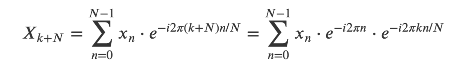
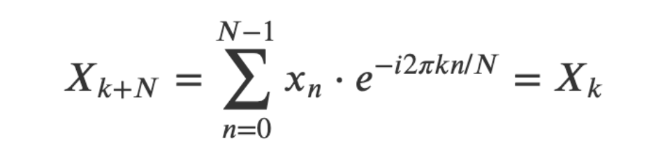
A question left unanswered in DFT is the symmetry. From DFT equation we can calculate this:
since $e^{-i2{\pi}n}=cos(2\pi{n})-i\cdot sin(2\pi{n})$ , $n$ is integer, so the cosine part is always 1. Meanwhile, the sine part is always 0. That made the equation above became
which means the symmetries will always happen.These symmetries essentially mean that certain calculations are redundant and can be eliminated.
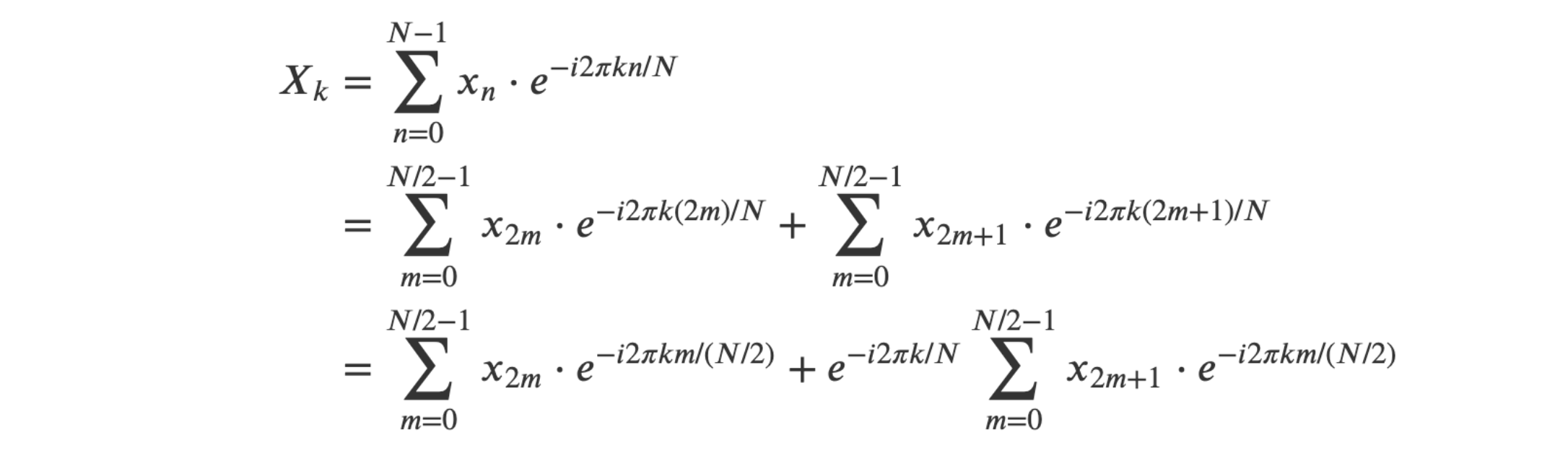
The concept of dividing DFT into smaller, even, and odd parts is a fundamental principle behind the divide-and-conquer strategy employed by the FFT algorithm (see equation expansion below).
By recursively breaking down the calculations into these smaller, more efficient steps, FFT significantly reduces the overall computation time required for large datasets.
While delving deeper into the mathematical specifics may not be my primary focus here, it's important to acknowledge the critical role these symmetries play in the efficiency gains achieved by FFT.
In life, people say don't be afraid of challenges, break down large problem into smaller ones, then you can tackle them easily. No matter who invented FFT, they must have mastered the philosophy of life.
Bins
The FFT algorithm employs a technique called windowing. It divides the original signal into smaller segments (often 1024 samples, chosen as a power of two for computational efficiency) and treats each segment as a short, repeating period. This windowing essentially isolates a small portion of the signal for analysis.
The simplest window function, the rectangular window, extracts this segment without any tapering or smoothing at the edges. Imagine multiplying the signal with a window function that's 1 within the segment duration (t=1) and 0 outside. This effectively isolates the desired portion, which is then treated as periodic by the FFT. Since FFT works best with periodic functions, windowing allows us to analyze the frequency content within that specific segment.
Similar to the concept of quantization in digital sampling, the continuous frequency spectrum is approximated in FFT. The spectrum is divided into discrete frequency bands called bins. The index k in the original DFT equation translates to the bin index in the FFT context.
The number of bins is typically half the window size (frame size). For a common frame size of 1024, you'd have 512 bins. The choice of sampling rate (44.1 kHz) is also relevant. With this setup, one frame represents a duration of approximately 23 milliseconds. The DFT computation is performed on the signal within this 23ms window.
Given the standard sampling rate covering 0-22.05 kHz (Nyquist point) and 512 bins, each bin represents a frequency resolution of about 43 Hz. This resolution works well for higher frequencies but may not be as accurate for lower frequencies within the spectrum.
Leveraging FFT in Python
In practical applications, obtaining bin information from an FFT is often straightforward. Libraries like NumPy's FFT package provide convenient functions for this purpose. The fftfreq function, for example, takes the window size (n) and sample spacing (d) as parameters and returns an array representing the center frequencies of each bin. This simplifies using FFT by readily providing the frequency scale associated with the calculated bins.
While the FFT analysis divides the frequency spectrum into linear bins, it's important to remember that human hearing perceives frequency logarithmically. This means we are more sensitive to changes in lower frequencies compared to higher ones. The equal spacing of bins in FFT doesn't directly correspond to how we experience sound.
To address this limitation, other time-frequency transforms have been developed. One such example is the Mel-frequency cepstral coefficient (MFCC) transform. MFCCs aim to mimic human auditory perception by using a warped frequency scale that approximates how our ears perceive pitch.
A crucial concept in FFT analysis is the trade-off between time resolution and frequency resolution. As discussed earlier, the window size (frame size) plays a significant role in this balance. Choosing a larger frame size leads to a finer representation of the frequency spectrum. The bins become narrower, allowing for more detailed analysis of individual frequencies within the signal. However, a larger frame size comes at the cost of time resolution. We lose the ability to precisely track how frequencies change over shorter time intervals. Imagine a sound with a rapidly changing pitch. A smaller frame size would provide more detail about these variations, while a larger frame size might smooth out the transitions between different pitches.
B. Implementation using NumPy's FFT
Both NumPy and SciPy offer FFT modules with user-friendly functions. Here, I'll focus on the numpy.fft package for its simplicity.
The fft function within this package efficiently computes the one-dimensional n-point DFT using the FFT algorithm. Similar to my diy DFT function above, it takes an array-like signal as input and returns a complex array representing the transformed data. However, fft offers significant advantages in terms of speed and flexibility.
One key feature is the optional n argument, which specifies the length of the output. This allows us to truncate (if n is shorter than the input signal length) or extend (zero-pad to reach the desired length if n is longer than the input signal length) . With the power of NumPy's FFT, I can now analyze complex sounds without worrying about excessive computation time. To demonstrate this capability, let's generate a richer sound with harmonics for spectral analysis.
import IPython.display as ipd
def harmonics(freq_bs, amps=[1.0], dur=1.0, fs=44100):
"""For a given fundamental frequency, create a harmonic series.
freq_bs = fundamental frequency
amps = list of amplitudes for each frequency in harmonic series.
The length of the list determines the number of harmonics.
dur = duration of the sound
fs = sampling rate, 44100 as default
"""
t = np.linspace(0, dur, num=int(fs*dur)) #create time sequence first
sound = np.zeros(len(t)) #a container for signal data
for i,amp in enumerate(amps): #extract each amp for each harmonic
harmonic = amp*np.sin(2*np.pi*(i+1)*freq_bs*t) #harmonic frequencies
sound += harmonic
return sound
fs = 44100
dur = 1.0
amps = np.random.random(6) #generate a random series of 6 numbers that valued (0~1)
sig = harmonics(220,amps,dur,fs)
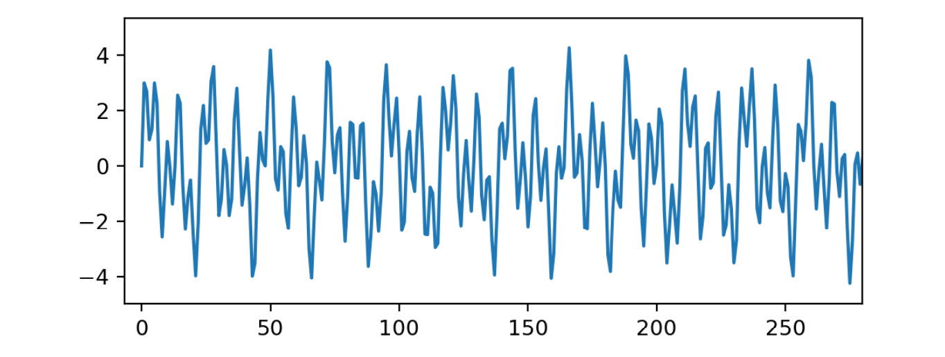
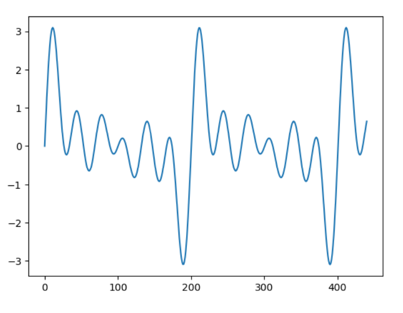
plt.figure()
plt.plot(sig[:441]) #about two cycles or more
plt.show()
ipd.Audio(sig,rate=fs)
a two-cycle segment of the soundwave
a sound with a 220Hz fundamental frequency will have a cycle of 1/220 second which is about
$1/220*44100\approx200$ samples.
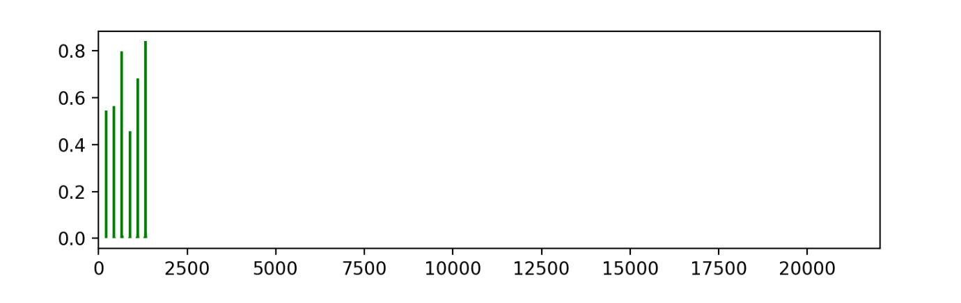
Next, to implement fft on the sound and plot the result:
X = np.fft.fft(sig)
N = len(X)                #number of frequency domain sampling
fft_bin = np.arange(N)    #bin index
freq = fft_bin/N*fs       #freq index

plt.figure(figsize=(8,3))
plt.stem(freq, np.abs(X)/N*2,linefmt='green', markerfmt=" ", basefmt=' ')
plt.xlim(0,N/2)
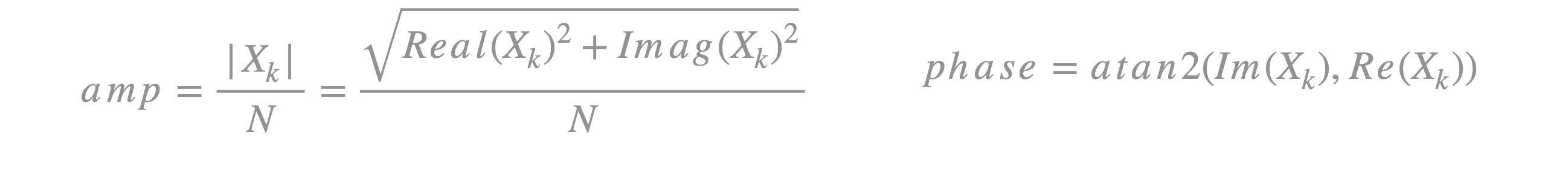
[notes] The result of DFT is a complex number includes amplitude and phase data of a component (complex sinusoid) of input signal . The formulas are derived from DFT equation:
Next, use inverse fft to recover the signal to exam the validation of fft function.